Improving performance
[1]:
%matplotlib inline
# dask and distributed are extra installs
from dask.distributed import Client, LocalCluster
import matplotlib.pyplot as plt
import mdtraj as md
traj = md.load("5550217/kras.xtc", top="5550217/kras.pdb")
topology = traj.topology
Much of the core computational effort in Contact Map Explorer is performed by MDTraj, which uses OpenMP during the nearest-neighbors calculation. This already provides excellent performance for a bottleneck in the contact map creation process. However, Contact Map Explorer also has a few other tricks to further enhance performance.
Dask
For multi-frame contact maps and contact trajectories, Contact Map Explorer can use Dask to parallelize across frames. Note that Dask is not required to install Contact Map Explorer, so you must install Dask separately to benefit from it.
When using Dask, a few things are different:
- You need to provide a
distributed.Clientto theDaskContactFrequencyorDaskContactTrajectory. - You need to provide the filename (and any other arguments needed by MDTraj, instead of the trajectory itself.
Dask might not give any performance boost on a single machine, but can be very useful if parallelizing across multiple machines. Because this directly takes a Client, it is easy to interface this with tools like dask-jobqueue.
[2]:
from contact_map import DaskContactFrequency, DaskContactTrajectory
from distributed import Client
client = Client()
client
[2]:
Client
|
Cluster
|
[3]:
%%time
freq = DaskContactFrequency(
    client=client,
    filename="5550217/kras.xtc",
    top="5550217/kras.pdb"
)
# top must be given as keyword (passed along to mdtraj.load)
CPU times: user 312 ms, sys: 30.3 ms, total: 342 ms
Wall time: 3.62 s
[4]:
# did it add up to give us the right number of frames?
freq.n_frames
[4]:
101
[5]:
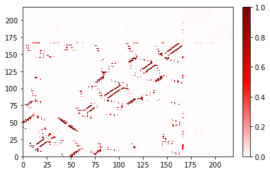
# do we get a familiar-looking residue map?
fig, ax = freq.residue_contacts.plot()
The same can be done for a DaskContactTrajectory. Here, we use the data from and compare to contact_trajectory.ipynb
[6]:
traj_2 = md.load("data/gsk3b_example.h5")

topology_2 = traj_2.topology
yyg = topology_2.select('resname YYG and element != "H"')
protein = topology_2.select('protein and element != "H"')
[7]:
%%time
dctraj = DaskContactTrajectory(
    client=client,
    query=yyg,
    haystack=protein,
    filename="data/gsk3b_example.h5",
)
CPU times: user 389 ms, sys: 26.8 ms, total: 416 ms
Wall time: 1.23 s
[8]:
# did it add up to give us the right number of frames?
len(dctraj)
[8]:
100
[9]:
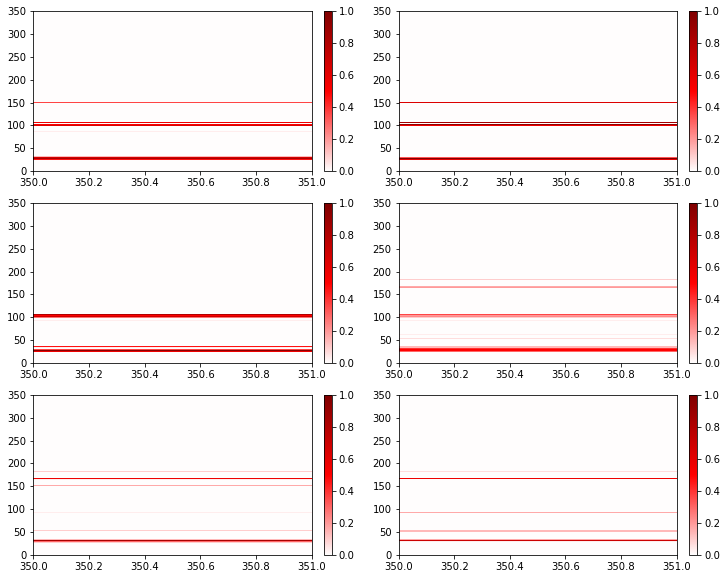
# do we get a familiar-looking residue map for rolling averages?
rolling_frequencies = dctraj.rolling_frequency(window_size=30, step=14)
rolling_frequencies

fig, axs = plt.subplots(3, 2, figsize=(12, 10))
for ax, freq in zip(axs.flatten(), rolling_frequencies):
    freq.residue_contacts.plot_axes(ax=ax)
    ax.set_xlim(*freq.query_residue_range);
“Atom slicing”
One of the internal tricks to improve performance is that we take the MDTraj trajectory that has been provided, and shrink it down to only the atoms that are included in the query and haystack. We refer to this as “atom slicing” (following terminology from MDTraj, although for performance reasons we actually implement it internally).
In most cases, you will want to atom slice. However, there are some cases where atom slicing can slow down your analysis – mainly if the atoms needed for the contact map are almost all the atoms in the trajectory. For this, you can turn atom slicing off.
[10]:
from contact_map import ContactFrequency
[11]:
# use all the atoms except atom 0
used_atoms = list(range(1, topology.n_atoms))
[12]:
%%time
# with atom slicing
frame_contacts = ContactFrequency(traj[0], query=used_atoms,
                                  haystack=used_atoms)
CPU times: user 267 ms, sys: 15.6 ms, total: 283 ms
Wall time: 118 ms
[13]:
# disable atom slicing
ContactFrequency._class_use_atom_slice = False
[14]:
%%time
# without atom slicing
frame_contacts = ContactFrequency(traj[0], query=used_atoms,
                                  haystack=used_atoms)
CPU times: user 392 ms, sys: 2.21 ms, total: 394 ms
Wall time: 234 ms
Note that this example is the worst case: the overhead for atom slicing occurs only once for an entire trajectory. However, if you’re generating many single-frame contact maps, this could be relevant to you.